D3 Zoom - The Missing Manual
How to zoom and pan in your data visualizations using SVG and Canvas


The best opening paragraph for a D3 zoom article has already been written and it goes like this:

It's good. In four sentences, it tells you precisely what zooming is, does and — probably more importantly — it takes your zooming fear. So, has it all been said then? Well, it never has. It’s always good to have numerous differing perspectives especially with events that move your precious visual all over the shop and scale it around at your trigger-happy user’s discretion.
A while ago, I worked on a fairly complex visualisation with many moving elements and a long list of interactions, including zoom and pan at its initially dark heart. The static visual itself was already relatively complex, but adding zoom and pan to it felt a bit like tying my son’s 4 by 6 foot Lego castle onto a fleeing water buffalo.
The conceptual problem here is, that zoom and pan so fundamentally interferes with our work. It appears to control quite a bit of our handcrafted visualisation, which is rarely ever a single whole thing, but a careful concoction of positions, scales and axes. This can be confusing at best and intimidating at worst.
So, after my zoom and pan moves grew in confidence, and were tested in a few other projects, the time seemed ripe to write them down. Maybe it’s too late and you all cracked it years ago, but even then, it might be helpful to have another perspective.
There will be three parts to our journey:
- A synchronous recipe for zoom and pan
- Building a visual
- Implementing zoom and pan in SVG and in Canvas
As a bonus, we’ll add programmatic zoom and make our visual pretty.
Now, you might look to that scroll bar over there, thinking you’ll miss supper when reading all this. It’s detailed for a reason, but I’ll make it easy for you to browse and cherry pick as I point out sections you can jump over without missing crucial stuff. So you can make this ride as short or thorough as you like and get something out of it either way.
A simple zoom and pan recipe
This first part is this post’s spine. It’s a short manual — nothing more than a series of five simple points you can follow while building up your zoom and pan events. This manual will give you a lifeline-like sequence of how to integrate zoom and pan into your app. The asynchronous and knotted world of programming is often helped by a series of synchronous and simple steps to follow.
Agreeing on some terminology
Before we pull ourselves along the line, let’s first define some helpful terminology:
A zoom transform is an object produced and maintained by D3. It’s your most valuable possession in the zoom and pan context, and it holds three values: the x and y translation as well as the scale factor represented by k. We shall see when and where it gets produced and changed very soon. This is how it looks in its initial state:

This says: “The user has not yet zoomed, or panned the visual. Therefore, the zoom-scale factor is 1 and x and y translation is 0.”
The zoom behaviour is the event system that keeps track of and passes on the transform values. A listener consumes (takes note of) the user’s actions. Once activated, it will send an event object with information about this event to a handler function. You will write this handler and use the information of the event object. The most important piece of information your zoom handler will receive is the above transform at every zoom activity. Whatever we want to do with the transform values, we will do in the zoom handler. This might sound like a lot, but in its simplest form you set the zoom behaviour up like so:
var zoom = d3.zoom().on(‘zoom’, zoomed);
The zoom base is the parent element the zoom is attached to or registered on, as they say. It does two things: 1) It’s the surface that takes in all the user’s moves and gestures, and 2) it holds the transform object (the x, the y, and the scale factor k).
The zoom targets are all the elements we want to move around. If you want to zoom in and out of a circle, then this circle would be your zoom target.
Furthermore, we might want to distinguish between two types of zoom. They will become much clearer when we move to our examples, but it will be helpful to define them on a top-level first:
Geometric zoom (or graphical zoom) means elements just get scaled up or down without any differentiation. All their properties will get scaled up or down. Think of it as moving or scaling the coordinate system of the respective elements. Everything on it will be scaled and moved indiscriminately. Geometric zoom is closest to our real-life experience. When we walk towards a house, each aspect of the house appears larger at each step. Equally, if we scale an axis all parts of it would become larger or smaller — the lines, the domain path, the labels. For example, a 14px axis label scaled up by a scale factor of 2 would appear 14 × 2 = 28px large.
Semantic zoom (or non-geometric zoom) means we control each single element’s property during zoom. If we have an axis, for example, with labels of size 14px and we semantically zoom in to the axis, we could command the labels to retain their original size for every scale factor. The lines might become larger and thinner and the axis would be repositioned according to the zoom, but our label would remain 14px large.
We won’t touch on this in the following, but bona fide semantic zoom can go further. It allows us to not only control the element’s properties, but the representation of our element depending on the zoom level. Google maps for example shows countries when zoomed out, states or administrational districts at medium zoom and smaller cities when zoomed in.
Zoom and pan in 5 steps

We are well-equipped for this now. Here’s our zoom and pan in five simple steps:
Build your static visual first
In order to zoom into a visual, you will need a visual.
Identify your zoom base and your zoom targets
Take a piece of paper, nominate an element that listens (the zoom base), and write down a list of elements that should move (the zoom targets).
Choose your zoom base element first. Determine which DOM element you want to use for your zoom base. You can attach the zoom to an
svg,g,rector any other element that your mouse has access to.Note here, that
gelements can only register events where they have children with a fill. So, if you have a largegelement with a circle of radius 1, your zoom gestures will only work on that tiny circle.It is often best to set-up a dedicated SVG rectangle (
rect) with fill but 0 opacity and pointer-events set to all to register the zoom listener on. You might have to unset pointer events of ascendant elements.Identify your zoom target elements and write them down. Remember, the zoom targets are the elements you want to move. Make a list of all zoom target elements.
For each target, identify if you want to use geometric or semantic zoom. Note it down. Here’s an example table you might end up with:
Function Element Zoom Type Scale props Zoom base rect#listener-rect - - Zoom target circle.planet semantic only circle radius Zoom target x axis tick lines semantic no Zoom target x axis tick labels semantic no
Set up the zoom behaviour
Now you want to set up the behaviour that will make the listener listen.
Create the zoom behaviour with at least:
var zoom = d3.zoom().on(‘zoom’, zoomed);
Check out the D3 API reference for d3.zoom() for helper methods like
scaleExtentandtranslateExtent.Call the zoom behaviour on your base element like:
zoomBaseElement.call(zoom)Note, you don’t have to call your zoom base
zoomBaseElementof course.
Write the handler
This is where the zoom and pan will happen. The handler’s single most precious possession will be the
transformobject updating x, y, and k continuously when the user wheels or drags. You will apply these to your zoom targets.The first thing you want to do is capture the
transformobject passed into the handler by the listener at every user interaction (wheel or mouse):var transform = d3.event.transform
Now that you have all 3 values, you need to do whatever you want with it: tx, ty and the scale k.
If you only want to administer geometric zoom, you just call:
zoomTargetElement
  .attr(‘transform’,
        ‘translate(‘ + transform.x + ‘, ‘ + transform.y + ‘)
          scale(‘ + transform.k + ‘)’);
or simpler:
zoomTargetElement.attr(‘transform’, transform.toString());...which is exactly the same. This assumes you want to apply all transform values. You can also focus on only tx, ty and the scale k of course.
If you want semantic zoom you need to rescale.
Assuming all your data values went through a scale to be translated from data to screen space, this translation changes on zoom. If your data point x = 10 was translated to pixel space 50 before zoom, the zoom will move it to a different point.
If you for example translate the x by 5 and scale by 2, the new position will be:
x2 = x1 × k + tx
x2 = 50 × 2 + 5 = 105
Luckily, you don’t have to (nor should you) produce these calculations yourself, but you can rescale your scale on each zoom and apply it to the target properties you want to change. These include axes or circles or rects or whatever target shapes and components you have.
With a scale called
xScale, you can use the sugar function.rescaleX()and apply it like so:var updatedScale = transform.rescaleX(xScale)Now you can use
updatedScalein your zoomed function for all the elements you want to update. For example an axis:xAxis.scale(updatedScale) gAxis.call(xAxis)or a set of circle x positions:
circles.attr(‘cx’. function(d) { return updatedScale(d.value); })
Do you need to programmatically move your target into a position?
First, determine the new positions tx and ty and the new scale k in D3’s own transform producing function by saying:
var t = d3.zoomIdentity.translateBy(tx, ty).scale(k)Store the object in the zoom base AND propagate the changes by calling your first zoom handler, which will move the targets with:
zoomBaseElement.call(zoom.transform, t)Now enable user triggered zoom with:
zoomBaseElement.call(zoom)
Here you are. I think they call this an executive summary. However, we have only superficially touched on the key concepts and haven’t even mentioned different renderers. Let’s add some flesh to the bones with a real life example.
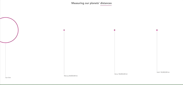
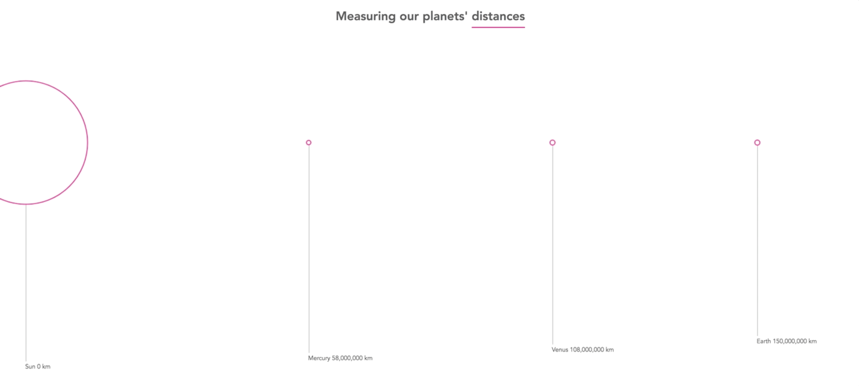
What we make
Here’s the Guinea pig we shall build in passing:
It’s a visualisation of our solar system’s planets showing their distance from the Sun. Zooming will come in handy to allow an overview and panning conveys some feel for distance. In addition, all orbs are pink!
Oh, and you don’t really have to, but if you want, you can follow along. Go here for all commented code. Alternatively, you can just play around with the app step by step. I’ll drop a link whenever we progress...
Building a static visual
As with nearly all visualisations, data is our starting point. So, here it is in its entirety:

We have 8 planets, 1 star called Sun, and Pluto, which is not actually a planet anymore but still in here for romantic reasons. We also have each planet’s distance from the sun and their radii. That’s all we need. But in order to turn it into this:

...we need to write some code.
Please note: this post is about zooming rather than about building a static visualization of our solar system. Nevertheless, I will run through the code to give you a round-trip of this app. However, if you’re only here for the zoom, please feel free to browse through this section and quickly move on to the first zoom-building step called Identifying our zoom base and zoom targets (mind you, it might be worth reading the Calculating the Dimensions section in a moment).
Let’s start with the sparse HTML:
<h1 id="headline">Measuring our planets'
  <span id="pink">
    <a href="https://en.wikipedia.org/wiki/Solar_System#Distances_and_scales">distances</a>
  </span>
</h1>

<div id="vis"></div>
That’s it. We have a headline with a link and a span to give it an appropriately pink bottom border and a container div for our vis. Moving swiftly on to the JavaScript bypassing the CSS which is not invited until the end of this post...
The first thing we do is to load in the data:
d3.csv("planets.csv", row, function (error, data) {
  if (error) throw error
  console.log(data)

  make(data)
})

function row(d) {
  return {
    planet: d.planet,
    distance: +d.distance,
    radius: +d.radius,
  }
}
We’re loading in our planets.csv piping it through the row() function which makes sure our numbers are indeed numbers. Then we call the make() function, which will be the home of all further code.
The make() function does the following...
- It sets the dimensions of our visual,
- it builds an
svgas well as a zoom surface, - it calculates our scales,
- it builds our axis, and finally,
- It builds the planets.
Let’s start with setting our visual's dimensions.
Calculating the dimensions
The margin and the height calculations are straight forward:
var margin = {
  top: window.innerHeight * 0.3,
  left: 50,
  bottom: window.innerHeight * 0.4,
  right: 50,
}
var height = window.innerHeight - margin.top - margin.bottom
We want the svg element to cover our entire screen. So our height will be the window.innerHeight subtracting some margins. We define the top and bottom margin in respect to the window.innerHeight to keep them relative to each other.
On to the width, which needs just a little more thought:
var maxDist = d3.max(data, function (d) {
  return d.distance
})
var mapScale = 1 / 10e4

// The full width of all planets
var chartWidth = maxDist * mapScale

// svg width will only be as large as screen
var screenWidth = window.innerWidth - margin.left - margin.right
The gist of our width calculation is that we want two widths. One for the chart and one for the svg. What’s the difference? Well, the chart will be very wide, because it needs to fit all our planets on it. The svg, however, doesn’t need to be very wide. The svg’s task is to show us the planets that fit on our browser window. An svg of the window’s dimensions is henceforth enough. It’ll look like this:

Note that this is only possible using the zoom behaviour. If we wanted to allow the user to see all planets without the zoom and pan magic, we would need to have an svg as wide as the chart. As a result, the browser would give us scroll bars, our users can use to move it to the right or left, like in the marvellous If the Moon were only 1 Pixel visual.
However, using D3 zoom, the zoom transform object we will initialise soon, will keep track of our gestures: how far we ‘scrolled’ to the right, the left and along the z-axis virtually piercing through the screen following our line of sight. Based on the transform we can re-position our elements and if they happen to be within screen coordinates, they get displayed on our base svg. No harm done if not, they just won’t get shown.
As such, our svg’s width will get the screenWidth which is just the window.innerWidth minus the margins. How wide will our chartWidth, the base for all planets be? We will scale down the distance between the two furthest apart orbs (the Sun and Pluto, that is) with our mapScale by 10e4 or 1:10,000. When Pluto is 5,913,000,000 km away from the Sun in real space, it will be 59,130 pixels away from the centre of the Sun in our visual.
That wasn’t too bad. Onwards...
Building out the base
First, we build our svg base: a margin-transformed g element dangling off an svg element:
var svg = d3
  .select("#vis")
  .append("svg")
  .attr("width", screenWidth + margin.left + margin.right)
  .attr("height", height + margin.top + margin.bottom)
  .append("g")
  .attr("class", "chart")
  .attr("transform", "translate(" + margin.left + ", " + margin.top + ")")
Then we overlay it with a rect element that we’ll use as our seonsor, our zoom base. This rect will listen to all mouse events and gestures and as such we’ll boldly call it listenerRect:
var listenerRect = svg
  .append("rect")
  .attr("class", "listener-rect")
  .attr("x", 0)
  .attr("y", -margin.top)
  .attr("width", screenWidth)
  .attr("height", height + margin.top + margin.bottom)
  .style("opacity", 0)
Important to note here that our zoom base is at the same spot as the zoom targets — the elements we want to zoom. We will attach our zoom base listenerRect to the svg (which in fact is the margin translated g.chart element as you can see just one code block above), which also be the home of our planet circles we’ll draw later.
Scales next...
Setting up our scales
We are mapping two measures to screen coordinates: distance and radius. As such we need two scales. Here's the first, mapping our planet's radii in km to screen radii:
var rExtent = d3.extent(data, function (d) {
  return d.radius
})

var rScale = d3
  .scaleLinear()
  .domain([0, rExtent[1]])
  .range([3, (height / 2) * 0.9])
First, we get the radius scale. We calculate the domain and map these values to a range of 3px to a little less than half our window’s height, keeping the measures relative to the window.
Our second scale is the distance scale:
var xScale = d3.scaleLinear().domain([0, maxDist]).range([0, chartWidth])
We map the data extent to the full chartWidth. If you mapped it to the screenWidth, all the planets would stand on their feet:

We could correct this by using a tighter radius scale, but we would like them to stretch out initially and then allow the user to zoom in or out.
Drawing the axis

We’ll be using a normal D3 axis component to build the axis. However, as you can see in the image above we will stagger the labels, so they don’t overlap.
First, we build out the axis component:
var xAxis = d3
  .axisBottom(xScale)
  .tickSizeOuter(0)
  .tickPadding(10)
  .tickValues(
    data.map(function (el) {
      return el.distance
    })
  )
  .tickFormat(function (d, i) {
    return data[i].planet + " " + d3.format(",")(d) + " km"
  })
We determine the exact number of tick mark labels by passing an array of the planets’ distance values to .tickValues(): [0, 58000000, 108000000, 150000000, 228000000, 778000000, 1429000000, 2871000000, 4504000000, 5913000000]. The axis will now only draw tick labels for these values. We use .tickFormat() to specify what the label will say. In our case, it’ll be planet name, distance from sun and km.
Now we produce the axis' g base and unleash the component on it:
var xAxisDraw = svg
  .insert("g", ":first-child")
  .attr("class", "x axis")
  .call(xAxis)
Like our listenerRect, the axis becomes a child of our g.chart element we labelled svg. Why insert it? We want our zoom base to be on top of all other elements dangling off the svg. so it can consume all the events. Looking at the DOM it should be the last child element of svg. To achieve this we’ll insert the axis — and soon the planets — before listenerRect.
Moving on to our axis labels. By default, all labels will be drawn on the same y level of course. But we want them staggered, so we need to write some code to achieve the steps. This is the stagger voodoo we apply:
// Move the axis-labels and -lines down
var labelHeight = xAxisDraw.select("text").node().getBBox().height
xAxisDraw.attr(
  "transform",
  "translate(0, " + (height + labelHeight * data.length) + ")"
)

// Position the axis text
xAxisDraw
  .selectAll("text")
  .attr("y", function (d, i) {
    return -(i * labelHeight + labelHeight)
  })
  .attr("dx", "-0.15em")
  .attr("dy", "1.15em")
  .style("text-anchor", "start")
Don't feel obliged to follow me down this rabbit hole — in short, we move them all down by # of labels × their label height. Then we move each label up by their height × their index. As a result, the Sun, for example, won’t move up as it'll be lifted by 0 × labelHeight = 0, but Mercury (the next planet to the Sun) will move up by 1 × labelHeight and so on.
The tick line needs a little more attention as we have to cater for its y1 and y2 value:
// Draw the axis lines
xAxisDraw
  .selectAll("line")
  .attr("y1", function (d, i) {
    return -(i * labelHeight + labelHeight)
  })
  .attr("y2", function (d, i) {
    return -(
      i * labelHeight +
      labelHeight + // this label’s start position from axis-y 0
      (data.length - 1 - i) * labelHeight + // the distance from the start position to the bottom of the chart area
      height
    ) // the height
  })
Good news. We can now draw our planets in (nearly) a single D3 chain:
var gPlanets = svg.insert("g", ".listener-rect").attr("class", "planet-group")

var planets = gPlanets
  .selectAll(".planet")
  .data(data)
  .enter()
  .append("circle")
  .attr("class", "planet")
  .attr("id", function (d) {
    return d.planet
  })
  .attr("cx", function (d) {
    return xScale(d.distance)
  })
  .attr("cy", 0)
  .attr("r", function (d) {
    d.scaledRadius = rScale(d.radius)
    return d.scaledRadius
  })
First, we create a group for all our planets and make sure the listenerRect also covers these planets by inserting our g.planet-group before the rect.listener-rect. Then we join and enter() the data to our as yet virtual .planet's, which will manifest as circles with the respectively scaled distances as x positions and rScaled radii. So there:

Great! We have our visual. Now let’s get to the zoom...
Identifying our zoom base and zoom targets

It’s often a wise idea to start with thinking about what you want to do before a head first code plunge. Before setting up our zoom let's identify what and how we want to zoom and pan. We ask 3 questions:
- What will be our zoom base — the “sensor element” that we’ll use for the zoom?
- What will be our zoom targets — the elements that we will move?
- What type of zoom do we want for each element — geometric or semantic zoom?
Identifying our zoom base
Let’s choose our zoom base element first. You can attach the zoom to an svg, g, rect or any other element that your mouse has access to. Note here, that g elements can only register events where they have children with a set fill property. So, if you have a large g element with a circle of radius 1, your zoom gestures will only work on that tiny circle.
As such, it’s often wise to set up a dedicated rect with fill, but 0 opacity. You have to make sure that the zoom base can consume all events. So, it should either be on top of all other elements, or its pointer-events should be set to all while all other elements’ pointer-events are set to none.
In fact, we already totally decided to set up an extra rect element to listen to events. We wisely cached it in the listenerRect variable, which we can refer to upon set-up. Done.
Identifying our zoom targets
Now let’s identify our target elements and write them down. Which elements do we want to move when we zoom and pan? Let’s make a list:
- The planets
- The axis and all their elements (tick lines and tick text only; we’re not showing the axis path).
Now we know our zoom base and our targets, we want to make sure they share the same coordinate system at the initial zoom state — when no zoom or pan has happened yet. That’s why we attached the zoom base and targets (planets, axis) to the same g above.
This is going really well!
Identifying the type of zoom
Lastly, let’s decide how we want to zoom them — eometrically or semantically? First of all, this distinction only makes sense for zooming, not panning. We’ve defined it above but for the purpose of redundant completeness, let’s repeat that Geometric zoom is simple: all elements are just being scaled up or down uniformly. Semantic zoom is a little more elaborate as you can decide what you want to scale up or down.
In our case, we might want to scale up the size of the planets, but keep the line width at 4px. For that we would need semantic zoom. For our educational purpose, let’s implement both types! Why not?
Setting up the zoom
For any zoom we decide to implement, we will need to set it up first. You probably agree that it couldn’t be less complex:
var zoom = d3.zoom().on("zoom", zoomed)
Calling d3.zoom() will return an object and a function. As with many parts of the D3 API, the object allows us to configure the variables we use in the function. So what we do up there is configuring the use of the d3.zoom() function with a single method: .on() attaches a handler function called zoomed. zoomed will be called every time we zoom. This is where we’ll make the elements move.
We have two other zoom cycle events to trigger a function, start and end. It should be relatively easy to guess when they would trigger the callback.
We store the returned function in the creatively named variable zoom. Next, we can use this function as zoom(<listener-element>) or, as it’s more commonly done in D3 <listener-element>.call(zoom) like so:
listenerRect.call(zoom)
That’s great, but what does that mean? It means that the listenerRect is now the official home of our zoom. Our zoom base! At this very moment it has two things dangling off it: The .on() event and the zoom transform. If we console.dir(d3.select(‘#listener-rect’).node()) and check our attributes, we’ll find these two D3 properties at the very bottom of the list:

The __on object holds our listener information and the __zoom object is a transform object holding the 3 values, this post started with. The x and y translation when we zoom and pan and the scale factor k changing upon zoom. You can always come to your zoom base — the listenerRect for us — to query the current transform values. However, you don’t need to very often as the transform will be handily accessible in the event object from within our zoomed handler function. Right. For the love of our lives — let’s finally zoom.
Geometric zoom with SVG

We have our static visual. We’ve set up the zoom. We’ve attached it to the zoom base. Let’s finally decide which type of zoom we’re going for. Here’s the thing: axes should be zoomed semantically, you decide for the other elements. Going back to our zoom targets let’s decree this here in a table on a piece of parchment:

Now, let’s write the zoom handler:
function zoomed() {
  var transform = d3.event.transform

  gPlanets.attr("transform", transform.toString())
}
We’re not quite done yet, but this is the simplest zoom possible and will already move our planets. We cache the transform object that dangles off the d3.event object which gets passed in on every zoom and pan move in the variable transform. Then we move our planets by just updating the transform attribute of our circles. transform.toString() is just a convenience method the transform object gives us. It saves us typing out the transform attribute’s value. For the identity transform { k: 1, x: 0, y: 0 } it returns the string "translate(0, 0) scale(1)"
How will this look?
Very good! The planets are moving — the rest is not. We need to do 3 things to improve this:
- Let’s prohibit the planets from moving to the right (there’s no planet left of the sun, so it would be futile).
- Let’s also prohibit the planets from moving up and down.
- Move the scales.
1 and 2 are simple; we just manipulate the transform object before we use it like so:
function zoomed() {
  var transform = d3.event.transform

  transform.x = Math.min(0, transform.x)
  transform.y = 0

  gPlanets.attr("transform", transform.toString())
}
As a result, x is never higher than 0 and therefore we can’t move the thing to the right. Also, y will always be 0. The result does what we expect:
Next, let’s make the axis move semantically. Our axis consists of labels and of lines. We choose semantic over geometric zoom as we only want to change their position on zoom — not the label size or the line width.
The main positioning engine behind the axis’ elements — the thing that makes the labels and lines move — is the scale. And what does the scale do? The scale maps our data values to the width of our svg element. If we want to change a scale with D3 we usually update the scale’s domain and/or range. But as rescaling axes is such a common activity for D3 zoom, we have the rescaleX() and rescaleY() methods dangling off the transform object. It updates the mapping for us according to the zoom. Perfect syntactic sugar we can use to create an updated scale:
var xScaleNew = transform.rescaleX(xScale)
The next section is called Semantic Zoom with SVG and will carelessly open the hood of this rescaleX() method for much more detail. But for now, let's just use xScaleNew trustingly like so:
xAxis.scale(xScaleNew)
xAxisDraw.call(xAxis)
We update the scale of our xAxis and redraw the axis with our new axis component. The last thing we need to do to the axis is stagger our labels and lines again, as we’ve done above.
// Stagger the axis-labels
xAxisDraw.selectAll("text").attr("y", function (d, i) {
  return -(i * labelHeight + labelHeight)
})

// Stagger the axis-lines
xAxisDraw
  .selectAll("line")
  .attr("y1", function (d, i) {
    return -(i * labelHeight + labelHeight)
  })
  .attr("y2", function (d, i) {
    return -(
      i * labelHeight +
      labelHeight +
      (data.length - 1 - i) * labelHeight +
      height
    )
  })
Remember, all of this happens in our zoomed handler.
It works:
Semantic zoom with SVG
This headline comes a bit late. We have semantically zoomed our axis already. But now let’s also apply it to our planets and dive into the rescaling process. Here’s our updated prep table:

Semantic zoom of circles
First of all, why would we want to use semantic zoom on the planets? I guess above gif demonstrates the semantic need well. As the planets get smaller, their outline is near-impossible to see. With semantic zoom we will have control over which element properties change or remain. In our case, zoom should change the position as well as the size of our planets but the width of the outline stroke should stay constant at 4px.
What we do is simple:
function zoomed() {
  var transform = d3.event.transform

  transform.x = Math.min(0, transform.x)

  var xScaleNew = transform.rescaleX(xScale)

  planets
    .attr("cx", function (d) {
      return xScaleNew(d.distance)
    })
    .attr("r", function (d) {
      return d.scaledRadius * transform.k
    })

  // Zoom and pan the axis here (...)
}
First, we remove our geometric planet zoom. Then we grab our planets and instead of transforming them, we specifically only access their cx and the r attributes. The x position will be re-calculated with the updated xScaleNew and the radius just needs to be multiplied by the scale factor. No translation necessary here.
And that’s it:
However far we zoom in or out, our stroke remains at 4px allowing us to actually see our planets even if they’re fully zoomed out.
Understanding zoom rescale

Semantic zoom requires us to zoom and pan properties selectively. Our semantic planet zoom above only changed the cx and the r attribute, while keeping the stroke width at 4px. To specifically change cx, we needed to update our scale — the main positioning engine of our visualisation — so that it positions our elements according to the new transform.
As said, D3 offers the convenience methods rescaleX() and rescaleY() to update scales according to the transform. It’s of course perfectly fine to use these methods without knowing the inner workings, so please feel free to jump straight to the next section. But if you’re curious about how exactly the rescale happens, stay with me. There'll be images in colour, too.
We’ll use a real simple example. Let’s assume we only look at the x-dimension and we want to map a data space that covers a domain from 0 to 100 to a 1000 pixel wide screen. As such we have a data domain of [0, 100] we want to map to a width range of [0, 1000]. Our scale would look like this:
var xScale = d3.scaleLinear().domain([0, 100]).range([0, 1000])
Let’s also assume we have 1 circle with the data value 20, which would be mapped to the pixel value 200:

Easy. Now we zoom in so that our scale factor k will be 2. No translation, just zoom. As a result, our circle would move according to our zoom transform formula we started this post with: tx + x × k, which would result in 0 + 200 × 2 = 400:

Note, we’ve also scaled up its radius by 2. All good so far? Great.
In this case, we could just do our transform calculation for the circle. But it’s of course much simpler, more convenient and consistent to continue to use our scale. However, we need to update it as our data value 10 shouldn’t scale to 100px anymore but to 200px!
How do we do this? As we've done above, we just pass our xScale to the transform.rescaleX() function. This returns the respectivley updated newXScale, which we use on the circle’s data value to determine the cx position:
var newXScale = transform.rescaleX(xScale);

circle.attr(‘cx’, function(d) { return d.dataValue; }); // d.dataValue is from a fictitious dataset
But what exactly does this rescale do? Let's look at the code first before considering its logic. A rescale under the hood looks like so:
function rescaleX(x) {
  var range = x.range().map(transform.invertX, transform),
    domain = range.map(x.invert, x)
  return x.copy().domain(domain)
}
As you can see in the last line, it will return the original scale BUT with an updated domain. The range will remain as is. If you asked me before I looked at this code, I would’ve guessed D3 would update the range and keep the domain as is. Much more direct. But it’s the other way around. This makes sense as the pixel range is a more static concept. In our case, 1000 is the width of the screen — that won’t change upon zoom.
The (small) downside is that the new domain calculation is slightly more involved than a new range calculation would be. There are 4 steps involved in calculating the new domain at each zoom and pan move:
- We first take the range of our original scale. In our example that would be [0, 1000].
- We then apply the inverse transform to it, which will return [0, 500].
- Next we will use the scale's
.invert()method to find the data value associated with the range values 0 and 500, which will be [0 and 50] in our case. - Finally, we override the current x-scale domain with this new domain and return it.
But why? Let's consider this conceptually...
First, we calculate a new range by taking the inverse of our transform function for the x value. By now we know the zoom transform function for x is tx + x × k. Its inverse is (x - tx) / k.
If you never came across inverse functions, they are just the opposite — the reverse of their main function. If you had f(x) = 3 × x then the inverse is g(y) = y/3. Plugging 2 into the main function f(x) returns 6 — plugging this 6 into the inverse function g(y) returns 2 again. It reverses the process of the main function.
Why do we take the inverse on our range? We want to adjust the domain, but keep the range at [0, 1000]. The easiest way to get the updated domain is to first calculate updated range extent values (min and max) in order to derive the new domain extent values from.
Let's play this through with a single value. Let's take our maximum range value of 1000. Our current scale maps the maximum data value of 100 to the maximum range value of 1000 pixel.
What's the max range value when we scale by 2? Scaling by 2 means we're zooming in. So, our current max range value of 1000 will move to 2000 (0 + 1000 × 2). However, we would like to know the new pixel point that moves to the edge of our screen when we zoom. The previous point that was at 1000 and is now at 2000 is no help to us as it's beyond the screen area now. So, which point is at the edge of our window after we zoomed? Which point is our new maximum range value?
In order to get that point, we don't ask: where does our current max range value of 1000 zoom to? We ask, where does the new max range value come from! Logically, this is the opposite or the INVERSE question. Accordingly, we apply the inverse zoom transformation: (x - tx) / k. We plug in our previous max range value of 1000px, our tx of 0 and scale k of 2 to get: (1000 - 0) / 2 = 500.

We can now say that our new maximum range value would come from the pixel position 500.
Why did we do this again? Isn't this all a bit silly as we want to keep the range at [0, 1000] anyway? Yes. And no. It's not silly, because we don't use this new maximum range value in a new range input for our scale. We just use it to find our new maximum data domain value.
We take our original scale that mapped a data value of 0 to 0 pixel, a data value of 100 to 1000 pixel and all in-between values accordingly. Now we ask which data value maps to the pixel value of 500? For this simple case we can use our brain, or — much better — we use the .invert() method of our original x-scale. xScale.invert(500) will return 50 as probably expected.
Let's remember here that we still have our original range of [0, 1000]. All the range calculations we have done, were only done in order to get to the new domain. Our new x-scale, still maps the data value 0 to pixel 0 but now maps the new maximum data domain value of 50 to the loyally standing maximum range value of 1000.

Likewise, our circle center x value still has the data value of 10, which now doesn’t map to 100 but to 200. We successfully zoomed in, we did.
Well done! Now, onwards to Canvas. Same game — different board...
Geometric zoom with Canvas

We only have 10 circles on our site. However, there are of course a great many more orbs out there to visualise. Visualising more than 1000 of them might get you into render performance troubles, which you can attempt to cure with Canvas. Unlike SVG, Canvas produces a single bitmap of your drawing. 1000 planets on your screen will be drawn to a single DOM element, the canvas. In SVG 1000 planets will produce 1000 circle elements that the browser has to maintain, which affects performance. There’s a list of Canvas resources below if you want to know more, but don’t worry, you don’t need a Canvas degree to follow along.
We will change very little in our app. As a quick reminder, here are the main steps we’ve folowed to get here:
- Load data
- Calculate the dimensions of our visual
- Build the SVG base and the listener rectangle
- Calculate the scales
- Define and draw the axis
- Build the SVG visual
- Zoom
We’ll change points 3, 6 and 7 above and leave the rest unchanged. In fact, we won’t produce a pure Canvas drawing, we will draw the planets in Canvas and keep the axes in SVG. This is called Mixed-mode rendering and is really clever if you have axes to draw, which is wonderfully solved by D3 in SVG but can be a pain in Canvas. (Elijah Meeks dedicates a good section on Mixed-mode rendering in chapter 11 of his book D3js in Action)
Adding a canvas base
As with SVG we need a base to draw on. For Canvas we need two things, the canvas element and its drawing context — the tools we can use to draw on the canvas. Below our svg base we add the following Canvas base snippet:
var canvas = d3
  .select("#vis")
  .append("canvas")
  .attr("width", screenWidth + margin.left + margin.right)
  .attr("height", height + margin.top + margin.bottom)

var context = canvas.node().getContext("2d")
It’s often wise to skip the margin convention for Canvas (we don’t have a g we can move around), however, especially when drawing SVG axes we want to cling on to our margins.
We also want to overlay our canvas element perfectly over our svg element and its children, the planet g and the listenerRect. To achieve this, we need to give it the same size as the svg element and position the canvas absolute on top of the svg. Here’s our css:
canvas {
  position: absolute;
  top: 0;
  left: 0;
  pointer-events: none;
}
Notice that we also remove all pointer-events from our canvas so that the listenerRect receives all gestures. As a result, we have quite a few layers:

The g now only holds our axis, which we can view through our svg. The canvas will display our planets, but only the section in green above (the other planets are drawn here for completeness but will initially be invisible). The top level is the listenerRect consuming all pointer events and informing our zoom and pan.
Drawing the planet circles in Canvas
We remove the logic that built out the SVG planets and instead draw our Canvas circles. We will draw it in a single function. Let me first show you the code of this Canvas drawing function before running you through it. Here we go:
function drawGeometricCircles(data, transform) {
We pass our data and the transform. If we only wanted to build a static visual we wouldn’t need to worry about the transform, but zooming is very much our mission!
context.clearRect(
  0,
  0,
  screenWidth + margin.left + margin.right,
  height + margin.top + margin.bottom
)
Next, we access our Canvas context (we cached in the context variable) and run a method called .clearRect. You can surely guess what it does — it clears the canvas. We pass it the canvas dimensions, which will clear the canvas every time we call this function.
This is what we do with Canvas. Unlike in SVG where we have manifest nodes in the DOM for our circles, we only have a pixel image on our canvas. Instead of moving around a DOM node, we just remove the image we drew earlier and draw a new image with elements in slightly different positions. That’s Canvas, that is.
context.save()
Then we .save() the default and unchanged context, and we .restore() it in a moment after all drawing is done. This way we secure not only a blank canvas slate, but also a blank context slate whenever we draw a new planet.
context.lineWidth = 4
context.strokeStyle = "deeppink"
context.fillStyle = "white"
Next, we define our painting brushes. We want a line width of 4px, we want a stroke color of deeppink and a fill of white. These aesthetic properties will apply to everything we draw after we set them. Until we change them.
context.translate(transform.x + margin.left, margin.top)
context.scale(transform.k, transform.k)
Theese next two lines are the geometric zoom. We translate and scale the entire image we draw by the respective transform values.
  for (var i = 0; i < data.length; i++) {
    context.beginPath();
    context.arc(xScale(data[i].distance), 0, rScale(data[i].radius), 0, 2 * Math.PI, false);
    context.stroke();
    context.fill();
  }

  context.restore();

}
Finally, we draw the circles. If you haven’t seen much of Canvas yet, this might look a little raw. And indeed, D3 internalises this loop through the elements for us by joining the data to selections that we can subsequently access, position and style. With Canvas, we do this ourselves. We loop through the data, start a path, draw the path as a circle with the context.arc() method, and finally stroke and fill the path.
The rest is a piece of code. We just need to call it right here and then with our data and the identity transform, which is simply { k: 1, x: 0, y: 0 }:
drawGeometricCircles(data, d3.zoomIdentity)
Whenever we zoom we replace the code that moved our SVG planets with this:
drawGeometricCircles(data, transform)
I’ll spare you the gif as it looks exactly like what we’ve seen above with geometric SVG zoom. But the working implementation with code is just a click away at!
Semantic zoom with Canvas
Let’s celebrate our geometric zoom feat by getting rid of it. In fact, to achieve semantic instead of geometric zoom, we will just rename and change our draw function. We will call it appropriately drawSemanticCircles(). Changing from geometric to semantic zoom in Canvas requires the same high-level actions. Instead of translating and scaling the planet’s coordinate system we will change the planet’s positions and radius according to the transforms.
drawSemanticCircles() will clear our canvas and then draw all circles with drawCircle():
function drawSemanticCircles(data, transform) {
  context.clearRect(
    0,
    0,
    screenWidth + margin.left + margin.right,
    height + margin.top + margin.bottom
  )

  for (var i = 0; i < data.length; i++) {
    drawCircle(data[i], transform)
  }
}
drawCircle() will be run for each data element, taking the data element and the current transform:
function drawCircle(elem, transform) {
  var x = transform.x + transform.k * xScale(elem.distance) + margin.left
  var y = margin.top
  var r = transform.k * rScale(elem.radius)

  context.lineWidth = 4
  context.strokeStyle = "deeppink"
  context.fillStyle = "white"

  context.beginPath()
  context.arc(x, y, r, 0, 2 * Math.PI)
  context.stroke()
  context.fill()
}
We first determine the x and the y positions as well as the radius. Then we define the styles for our circles. Lastly, we draw our galactic spheres as arcs. And that’s it...
Great! We’ve covered the two types of zoom in two renderers. On to the bonus tracks: programmatic zoom and making our galaxy pretty...
Programmatic zoom
It’s often helpful to move our visuals into a certain position. You can let a user center a map, move a long bar chart to the beginning or zoom in and out of the solar system.
We have neither a map, nor a bar chart, so let’s programmatically zoom out and back into our planets upon load. We go back to SVG for this, as we don’t really need Canvas here. Because of its lower level, I’d recommend using Canvas only if you need it or speak it like your mother tongue. As we only have 10 circles to move around here, we don’t need it.
Here’s what we want to achieve:
We start with a heavily zoomed in visual at a zoom scale of 20. We then zoom out to our minimum zoom, so all planets fit comfortably on the page. Lastly, we zoom back in to our default zoom scale of 1.
To achieve this we bolt on the programmatic logic to the bottom of our make() function where all our app code lives. We start by zooming in to a scale factor of 20 without panning:
var initialTransform = d3.zoomIdentity.scale(20)
listenerRect.call(zoom.transform, initialTransform)
d3.zoomIdentity returns the identity transform we have already encountered a few times. We change the transform scale to 20 and cache it in initialTransform. Then we use the zoom.transform() function. This function is obviously different from our transform object, but it directly manipulates it. We use it here with D3's own <selection>.call() method we encountered above. The selection we call zoom.transform() on will be its first argument. It will be our zoom base listenerRect, home to our current transform object. The second argument has to be a new transform object. It will replace the current transform on that node.
The cherry on top is that instead of passing our zoom base as a simple selection, we can pass it as a transition. Remember (or note) that transitions are just derived selections, so passing in listenerRect.transition() will in fact transition our visual from one transform to the other.
But so far, we,ve just snapped our visual to a scale of 20. Let’s kick off the transition. First to a scale of minZoom we have defined earlier, then to a scale of 1. Here’s what we do:
// Trigger programmatic zoom
progZoom()
Let’s write it. It won’t take any arguments:
function progZoom() {
We first define the transform for the minZoom we want to zoom to first:
var zoomOutTransform = d3.zoomIdentity.translate(0, 0).scale(minZoom)
We define .translate(0,0) only to be overly clear that there's no translation here.
In the following lines, we turn our listenerRect into a transition and call zoomTransform() again. Using .call() we pass in the transition we just built as a first argument and zoomOutTransform — the minZoom transform we just saved:
listenerRect
  .transition()
  .duration(5000)
  .call(zoom.transform, zoomOutTransform)
  .on("end", zoomToNormal)
At the end of the zoom we call a function called zoomToNormal. Which is doing exactly what we just have done, apart from transition-zooming to an identity transform:
function zoomToNormal() {
  listenerRect
    .transition()
    .duration(3000)
    .ease(d3.easeQuadInOut)
    .call(zoom.transform, d3.zoomIdentity)
}
Apart from zooming to a different transform, we’re also setting a different duration as well as a different easing function.
}
And that was our first bonus track. On to track 2...
Making our visual pretty
It’s wise to get your visuals right in black and white first (pink and white in our case). But in the end a lick of paint can’t hurt. In order to get here...
...we only need to change a few things, of which the planet’s glow is probably the most elaborate. Let’s look at the rest first:
We’ll add a dark blue background with a radial gradient moving into the dark blue from a slightly lighter one. It’s one line in our body css:
body {
  font-family: Avenir, sans-serif;
  font-size: 0.75rem;
  margin: 0;
  background: radial-gradient(#091c33, #091426);
}
We change the text and line colour to a grey off-white (#ddd), and instead of the solid lines we render dashed lines with wide gaps:
.tick line,
.lines {
  stroke: #ddd;
  stroke-width: 0.5;
  shape-rendering: crispEdges;
  stroke-dasharray: 1, 5;
}
Lastly, we fill the planets in our favourite deeppink and add the glow. The glow is an SVG filter we apply to each planet. I won’t go into detail here but you can find the code commented right here. In short, we thicken the planets a little bit before feathering them with some Gaussian blur. We fill the blur deeppink and marvel at the resulting glow. The filter gets an id of #soft-glow, which our planets can reference with the filter attribute:
var planets = gPlanets.selectAll('.planet')  .data(data).enter()
.append('circle')
    .attr('class', 'planet')
    (...)
    .attr('filter', 'url(#soft-glow)');
And that’s it!
We’ve come a long way and hopefully now understand D3 zoom a little better. We’ve looked into a short recipe you can follow before and during wiring your visual up with any zooming and panning. We then applied this blueprint to a real project with pink orbs, playing through geometric and semantic zoom rendering in SVG as well as Canvas. As a bonus, we looked at programmatic zoom and finally made its subtly pink face even more pink. What fun!
This post should also end where it started: with the idea of having a life-line, a recipe, a step-by-step manual to follow when building out zoom and pan. As such, this bigger article has a little sister that is exactly that: 5 steps from no zoom to zoom (including programmatic zoom). Have a look... I implore you.
Two more things that might help: a quick note on updating your zoom from D3 v3 to v4 and a list of sources.
Updating zoom from v3 to v4
In 2016 (as in many generations ago) D3 v4 superseded v3 with some great but breaking changes. Some conceptual changes including the zoom behaviour kept devs up at night (including myself). The changes are consistent and sensible, but are worth a few extra notes that might help you find sleep:
- As with v3, zoom in v4 is just about the x and y translation and the scale — the transform parameters. That is, of course, brutally simplifying complexity, but it’s a mantra you should try out when gridlocked.
- The transform parameters are stored with the zoom base in v4, while they were stored with the behaviour in v3. The behaviour now just passes the transform on to the targets. This is good to know when we want to retrieve the transform outside of the zoom handler.
- The v3 behaviour rescaled your scale automatically. In v4 you need to rescale your scale in the zoom function manually and update all scale-based shapes and components. This is a little more work, but significantly less magic and a clearer separation of concerns.
Sources
There is no abundance of D3 (v4) zoom related posts and tutorials out there. The lack thereof was one reason to write this tutorial. However, there are a few zoom gems as well as some helpful further Canvas related material you can have a look at:
- A summary of this tutorial in the shape of a concise manual
- GitHub repo for all code we went through in this article
- All the steps we took above as working implementations
- Read this very post again on Medium (go on..)
- Zoom explained by Empty Pipes
- Zoom explained by Puzzlr
- Zoom with React and D3
- Mike Bostock’s zoom examples
- Geometric vs Semantic Zoom
- D3 v4 Zoom API Referene
- D3 and Canvas (shameless self-reference)
- More D3 and Canvas
- And even more D3 and Canvas
I hope you enjoyed reading this and please do say hello to just say hello or tell me about other ways to zoom. Knowledge is partial and we're all here to learn...
